Control theory for fun and profit

Fauna is a distributed system. Like all distributed systems, we have the somewhat vexing problem of an unreliable network and faulty nodes (not byzantine faulty, just the regular slow or dead kind). The chance that a faulty node received a share of work in a request is greatly amplified when the result of one request requires a combination of data from several nodes. In such a scenario that is common for a distributed system—a faulty node could impact many requests. Methods to increase the reliability of your system in the presence of faulty nodes are therefore indispensable.

Whenever you need to request data over a potentially unreliable link and multiple nodes have the data there is an easy method to turn a set of unreliable links into a single virtual link that is both more reliable and faster in the tail in aggregate than any one of the individual links. Just issue requests redundantly. The fastest path of the available paths will return first. Of course, issuing redundant requests has its own problems: increased server load for machines servicing the requests and increased network traffic for both parties.

Issuing redundant requests naively might increase network traffic and overload servers that were previously fine.

Instead of flooding the cluster with redundant messages in every scenario, we could try to determine when we have to send redundant messages. The most straightforward way to do this is to simply wait and see whether the result comes in fast enough. Instead of sending redundant requests right away, the node would wait for a specific delay and send a backup message when it did not receive an answer within the given time-frame.

In fact, almost all the gains of redundant requests can be had if we delay issuing the second request until we have waited out some high percentile of the response distribution. The Tail at Scale paper recounts how waiting out the ~ 98% percentile response time (they measured a fixed delay of 10ms) before issuing a redundant request reduced the 99.9th percentile from 1800ms to 74ms while only costing them a modest 2% extra utilization.

The Next Problem

This is all well and good in theory. There is, of course, an obvious pressing and practical concern: how does one figure out how long one should wait before sending the hedged request? Ideally, it’s small enough since each request that requires backup messages would take at least the time of the delay. But it can’t be too small either since the cluster would be flooded with backup messages. A simplistic and obvious answer is to measure it. We could determine the percentage of messages that we desire backup messages for, measure it directly, and adapt where needed.

Let’s say we aim to wait for the 98% percentile like in the paper. By gathering latency measurements for all our requests, we can determine the exact ‘backup request delay’ to make sure that only 2% of the requests trigger a redundant request.

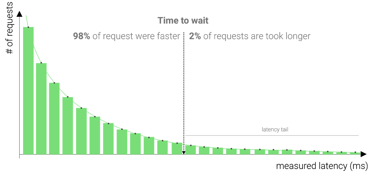
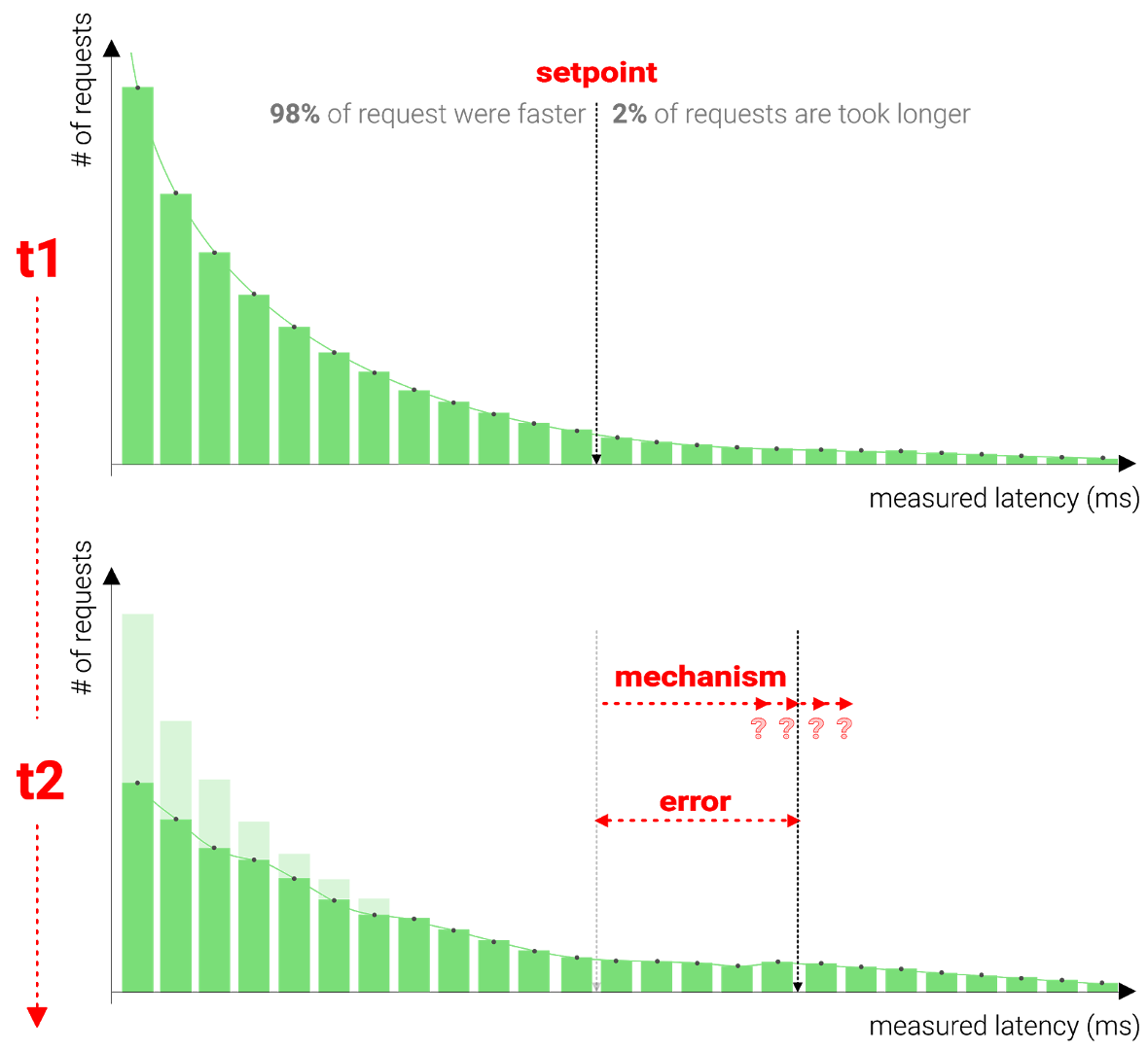
In reality, it’s much more complex, by the time we have set our delay based on our measurements, the latencies might have changed due to external factors. Additionally, by setting this delay, the measurements will change, influencing the measurements which we rely on to take action can have bad side-effects.

In a naive approach where we set the delay each time exactly according to our measurements, we might accidentally make things worse. If due to an anomaly such as a netsplit, our latencies are severely skewed for only a split second we might set an extremely high delay. Setting such a high delay might affect our measurements which then results in an even higher delay, which again has an effect on the percentile, which in turn results in a higher delay, which again results in … . . .

I believe you get the point, a system that acts in a loop where it takes action on measurements that are influenced by its actions could quickly go rogue instead of stabilizing on an optimal value. There are many bad scenarios to avoid:

• Slow convergence: the system takes too long to respond.
• Constantly in flux: the system continuously jumps up and down instead of stabilizing, typically caused by responding too quickly.
• Snowball effect: an anomaly results in a poorly chosen value which enforces the anomaly.

In essence, dealing with such a moving target raises even more questions: over what time slice should we measure? How should we evolve the time to wait if we measure the latencies continuously? Weighted average? Exponential? What weightings?

The ideal solution should react rapidly to changes in network conditions and converge to the right value without overshooting it. Now, in our case, getting this a little bit wrong either side isn’t the end of the world but it does have consequences: slow convergence or overshoot depending on the direction from which it arrives either means overly slugging request servicing or overconsumption of computing resources.

Control Theory To The Rescue

Fortunately, this kind of problem falls into a well-known area of study which is very common in electronics yet less often encountered in the wild in computer algorithms. In fact, the thermostat in your home has to solve similar issues. It needs to achieve a target by reacting to measurements that are influenced by its own actions (start heating) and external stimuli (an open door lets in the cold) in a constant loop.

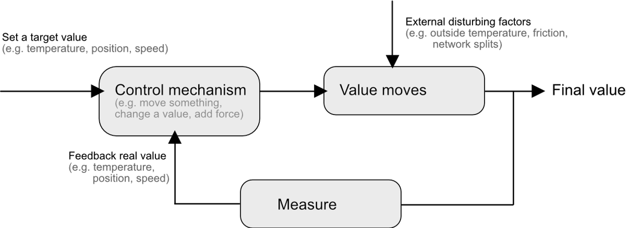
Check out this visual analogy where a motor is controlling the position of a ball in response to external stimuli. This system has to decide on a course of action based on measurements of a constantly moving target that is influenced both by external stimuli (the hand that moves the ball out of center) as well as its own actions (tilting the plate).

(source Giphy)

This plate controller is doing exactly what we’d like our software to do. It has a setpoint (keep the ball in the center of the plate), it has an error (the distance of the ball to the setpoint) and it has a mechanism for reducing the error (tilting the plate). Our setpoint is the ratio of requests that trigger a backup read to those that don’t, our error is just the gap between the observed ratio and the target ratio and our mechanic to influence this ratio is the delay before issuing the backup request.

How is the plate being controlled? With a PID controller.

PID Controllers

PID controllers are classic closed-loop control systems that every tick gather information and take action to bring the system to some desired state. PID is a mathematical answer to this type of problem that was invented in the 17th century to keep windmills running at a fixed speed.

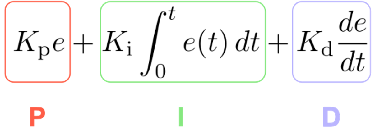
PID is an initialism standing for Proportional, Integral, Derivative which are the components used to tame the system and a PID controller is the embodiment of this function which has taken many forms over the years; mechanical (a pneumatic device), electrical (chips) and finally the programmatic implementation that can be used to optimize distributed systems.

The function combines the error (P), the accumulated error over time (I) and the predicted error (D) each multiplied by a tunable constant respectively. Why does this make sense?

By specifying a weight for these three factors (using the constants Kp, Ki, and Kd), we can finetune how our system should behave to prevent overshooting, accumulating errors or unstable situations.

• Proportional: we adapt the setpoint relatively to the size of the error. This is meant to trigger a fast reaction.
• Integral: take into account how the error has behaved over time which helps to remove a systematic error. The integral part receives more influence the longer the error accumulates over time. Which means that systematic errors will eventually be mitigated.
• Derivative: could be seen as the variable that predicts the future and helps to prevent overshooting the target. The derivative would slow down the process if we are moving too fast towards the target.

See this video series if you want to really dive in. This is exactly what we want: when our ratio is out of wack we want to safely yet rapidly change the delay to converge back to our desired state keeping the system responsive while minimizing resource usage.

Conclusion

The introduction of backup requests and a delay before we actually issue these requests was only the first step of the approach. By introducing the PID controller as a third element we can more readily adapt to delay when the circumstances change. With these three insights combined into one algorithm, we expect to retain all of the benefits of issuing backup requests while making fewer requests.